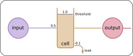
This page offers interactive figures for the paper "Integration of LIF neurons in Deep Learning Architectures".
The LIF Unit
\begin{aligned}
V_{t} &= w_\mathrm{input} \cdot x_t + (1 - w_\mathrm{leak}) \cdot V_\mathrm{t-1} \cdot \Theta(V_\mathrm{thresh}-V_\mathrm{t-1})\\
y_{t} &= \Theta(V_{t} - V_\mathrm{thresh})
\end{aligned}
The response of the leaky integrate and fire neurons. The cell integrates the input until the internal state
exceeds the threshold. Then it outputs a spike. The leak term lets the cell state decay over time.
Image processed columnwise by a LIF layer. The image displays the input, internal state or the output of the LIF layer.
Backpropagation of the error
For error backpropagation we treat the two $$\Theta$$ function in the LIF equations differently.
The $$\Theta$$ function used for the spiking
output ($$\Theta_1(x)$$) is defined with its derivative being always 1, while the $$\Theta$$ function for resetting
the membrance potential ($$\Theta_2(x)$$) is defined with its derivative being always 2.
\begin{aligned}
V_{t} &= w_\mathrm{input} \cdot x_t + (1 - w_\mathrm{leak}) \cdot V_\mathrm{t-1} \cdot \Theta_2(V_\mathrm{thresh}-V_\mathrm{t-1})\\
y_{t} &= \Theta_1(V_{t} - V_\mathrm{thresh})
\end{aligned}
with
\begin{aligned}
\Theta^\prime_1(x) = 1\\
\Theta^\prime_2(x) = 0
\end{aligned}
The response and gradient of a LIF cell. Each column represents one time step. The color saturation denotes the
value of the cells. On hover the colors denote the back propagated error from the selected time step.
Network Architecture 1
Layer (type)
Output Shape
Parameters #
LIF-Layer
(None, 400, 500, 3)
6
Reshape
(None, 500, 1200)
0
LSTM Layer
(None, 500, 30)
147720
Dropout
(None, 500, 30)
0
Time distributed Dense
(None, 500, 30)
930
Dropout
(None, 500, 30)
0
Softmax
(None, 500, 10)
310
Spiking network processes images. The network
takes images as input and applies a LIF layer to generate spike trains for each row and color channel. These spike
trains are fed into an LSTM layer which is followed by a softmax layer. The softmax layer predicts the category of the image. The categories are represented by images of the training data set, whereas the images used for illustration (input) are part of the test data set.
The three different colorbars (lif cell) represent the internal state of the LIF units for the three different color channels. The spike data is produced by this LIF layer is shown under the heading lif output.
The activation of the LSTM layer is shown as color map (lstm). The category probability calculated through the softmax layer is represented by the size of the category images (softmax).
Network Architecture 2
Layer (type)
Output Shape
Parameters #
Reshape
(None, 500, 1200)
0
TimeDistributed Dense
(None, 500, 1200)
1441200
LIF-Layer
(None, 500, 1200)
2400
LSTM Layer
(None, 500, 30)
147720
Dropout
(None, 500, 30)
0
Time distributed Dense
(None, 500, 30)
930
Dropout
(None, 500, 30)
0
Softmax
(None, 500, 10)
310
Training of a network with LIF units; The figure shows the spiking output of 1200 trained LIF units. Thus, the data was split in 3 blocks only for visualization.
Each block consists of 400 lines, which correspond to 400 LIF outputs. The x-axis is the time axis (for each block individually, each block consists 500 time points). The output of each LIF unit is a boolean scalar, which changes over time (x-axis).
The input of one LIF unit in each time step is a weighted sum of the rows of the image (each image has 400 rows and 3 color channels, input: weighted sum of 1200 values). It can be seen that the output spike patterns change during training and that the spike density is reduced.
Thus, the network develops a sparse coding of the input image.